“What’s making it so slow?”

That’s not an uncommon question in software development — users like software that reacts quickly and as engineers, that means an occasional need to dig into your code and figure out just where the culprit is.

Sometimes it’s easy to spot the problems — making too many database queries or using a slow external API. But other times, finding the root cause is much harder and that’s where some profiling knowledge can be hugely helpful.

This post will introduce some practical ways of finding bottlenecks in large real-world projects. We’ll have a brief look at Python’s built-in profiling capabilities, move on to visualizing the slow execution paths and finish with low-overhead profiling methods that you can run even on production servers.

Introduction to Profiling

Profiling basically means analyzing program’s execution and performance at run-time. It can be really simple, e.g. adding code to measure overall time spent in a function call. Such simplistic approach is easy to add and analyze, but provides very limited information — you’ll see how much time was spent in that one function, but not much more.

Much more useful approach would be one that analyzes your codebase as a whole, and then gives you overview of which function calls were the costliest, without having to specifically add profiling code to each and every one of them.

Profilers do exactly that — you’ll get a full picture of where time was spent during the analyzed period.

Quick bit of theory before getting to the more practical parts — there are two general types of profilers. First ones are event-based aka deterministic profilers. They work by using special hooks to monitor your program’s execution and tracking every function call event (and some others). Event-based profiling adds certain overhead to your program so using it in production isn’t advised. The upside is that it accurately tracks the program’s execution, giving you e.g. exact function call counts which might be useful.

The other group are statistical aka sampling profilers. These use a different approach of looking at the program’s current call stack many times per second. Given enough samples, you will get a statistically accurate-enough overview of which functions are used the most. The sampling interval is usually quite short — e.g. 1000 times a second — but the resulting overhead is nonetheless much smaller than that of event-based profilers.

We’ll be using a simple Django view from Discore for demo purposes. Discore is a web application for tracking discgolf games, built by some colleagues from Thorgate, and we’ll profile one of its API endpoints that makes a few database queries and contains a bit of business logic as well.

Python’s Built-in Profiler

Let’s begin with a quick look at Python’s built-in cProfile module. While being less advanced than some of the alternatives we’ll be looking at soon, it can nonetheless be useful for quick jobs. Being included in Python’s standard library is its big advantage as it puts the bar for trying it out really low.

We’ll profiling the get() method of a Django view by creating a Profile() object, wrapping the code we want to profile between Profile.enable() and Profile.disable() calls and finally displaying the collected info:

import cProfile as profile
import pstats

# Add profiling to a Django view
class ProfiledView(GameView):
    def get(self, request, *args, **kwargs):
        # Start the profiler
        p = profile.Profile()
        p.enable()

        try:
            # Run the code we actually want to profile
            return super().get(request, *args, **kwargs)

        finally:
            # End profiling and print out the results
            p.disable()
            pstats.Stats(p).sort_stats('cumulative').print_stats(30)

As a result, you’ll get statistics about the 30 most time-consuming function calls printed out. I won’t go into explaining the output format for brevity, but it’s not the easiest to quickly grasp, especially for more complicated programs (where profiling is most useful).

Although the cProfile module is very easy to get started with, it has problems with output complexity as well as overhead. The output does now give a very good overview of the program’s execution paths and finding hotspots can be difficult, especially for beginners. The built-in profiler also has noticeable overhead — in Discore code it was roughly 50%, but if your app has more logic inside the Python code and spends less time on database queries and other blocking operations, then the overhead would be even larger.

Check out profilehooks package as well — it makes using the built-in profiling functionality a bit easier by providing various decorators.

Yappi and Call Graphs

The textual output from Python’s cProfile module can be a bit… overwhelming. I personally find it much easier to grasp visual representations of data. Turns out there are a few tools that apply this mindset to profiling.

One of them is Yappi — and alternative profiler package that supports call graphs. Call graphs store more information for each function call — not just how many times the function was called or how long it took, but also the whole call stack, including the function that called this one. This means that graphical representations of program’s execution can be created. Combined with specialized tools for reading and visualizing this info, you can have an interactive graph showing where time was spent and you can drill down to the parts that interest you to see more info about them.

There are several call graphs visualizers available. You can search for “callgrind viewer” and find some. You’ll need something that understands Valgrind’s callgrind format. A good one that I use on Linux is KCacheGrind.

Using Yappi is very similar to the cProfile module. First, install it from pypi: pip install yappi. Next, let’s modify the previous example:

import yappi

# Add profiling to a Django view
class ProfiledView(GameView):
    def get(self, request, *args, **kwargs):
        # Start the profiler
        yappi.start()

        try:
            # Run the code we actually want to profile
            return super().get(request, *args, **kwargs)

        finally:
            # End profiling and save the results into file
            func_stats = yappi.get_func_stats()
            func_stats.save('callgrind.out.' + datetime.now().isoformat(), 'CALLGRIND')
            yappi.stop()
            yappi.clear_stats()

After running the profiled code, you should a file with name similar to callgrind.out.2018-01-25T12:09:39.973370. Open it with KCacheGrind or another callgraph visualizer and you should see something similar to this:

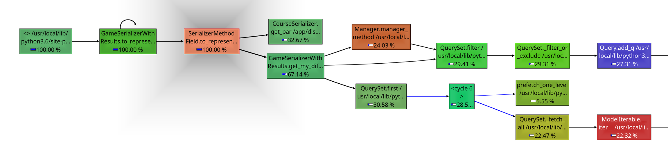
This looks pretty intuitive! You can see how the execution branches into two functions which are respectively responsible for 33% and 67% of the entire execution time. The graph is interactive and clickable — by clicking on one of the other nodes, you’ll see the call graph centered around that one. This makes it easy to get to the bottom of the problem and find the functions responsible for the most of the time spent.

Another nifty visualization mode is treemap. Treemaps can be a bit confusing at first, but they can be really good for visualizing hierarchical data. In our case, area of each rectangle on the graph corresponds to the amount of time spent there.

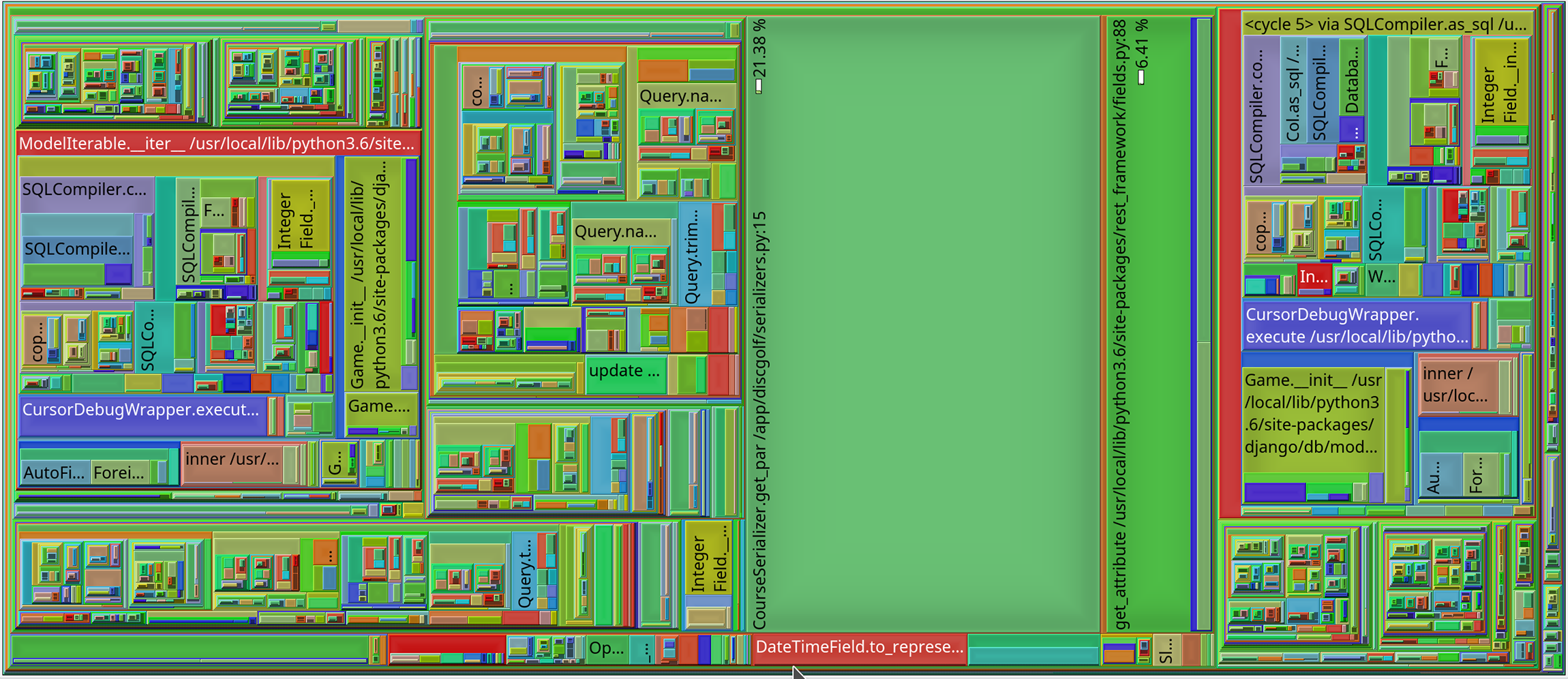
You can immediately spot a few big, ‘flat’ areas showing functions that don’t call any subroutines, but spend a lot of time nonetheless. You can also spot areas with high degree of nesting. These can be trickier to understand, but often correspond to complicated code in your framework / libraries, such as database access in Django or logging in Python standard library. As before, you can interactively drill down by clicking on any of the nodes.

If you’re unsure where to begin with the actual optimizations, it’s usually good to start with the functions where a lot of time is spent but that doesn’t make any further calls. In the treemap, those are the same big flat areas. If they’re in your own code, you might be able to rethink a few loops or calculations and save a lot of time. Another good starting point are the spots where you call an expensive function from a library, e.g. fetching database objects in Django. Sometimes these turn out to be unnecessary and you can again save considerable amount of time by rethinking your program flow.

So Yappi creates much more thorough results that can visualize the program flow and to some degree even visually explain what’s going on. Unfortunately it comes at a cost. Running code in Yappi is about 2.5x times slower for our example, and could be more in some cases.

For an alternative call-graph-generating profile, see pyinstrument. It comes with out-of-the box Django integration and optional sampling profiling mode, which could be useful.

Pyflame

So far, we’ve been looking at event-based profilers which continuously track program’s execution, recording every event such as function call. This is very accurate but comes with a rather heavy overhead.

I mentioned that there are also statistical profilers. These work by looking at the program’s current call stack at fixed intervals, e.g. 1000 times per second, and taking note of what your program is doing at that moment. This means that there’s no need to track every individual function call which reduces overhead a lot, and also means that the program doesn’t need to be modified for profiling.

We’ll take a closer look at Pyflame — a statistical profiler for Python, created by Uber. It has several nice properties. Working as an ‘external agent’, it requires no modifications whatsoever to your program’s source code. It is capable of generating flamegraphs — another good way of visualizing program’s execution —, and supports multi-threaded programs. Being a statistical profiler, it also has very low overhead, so you can use it even on production servers. Last but not least, Pyflame supports profiling Python programs running inside Docker containers.

A potential downside is that it only supports Linux.

Installation

Pyflame is a C++ program, requiring a bit of assembly. There might be pre-built packages available for your distro, and if you’re super lucky they might even be up to date (but probably not).

I found that it’s quite easy to use Docker for the compilation — that way I don’t need to install anything on my host OS and can target the exact Python version that my program’s running on.

Discore uses Python 3.6 so we’ll want Pyflame to be compiled against the same version (if you need a different Python version, just use the corresponding version’s Docker image). Let’s use the official 3.6.4 Python docker image and start a shell:

docker run -it -v /tmp/pyflame:/build python:3.6.4 bash

We mounted /tmp/pyflame into the container as /build directory, so that we can easily retrieve the compiled executable — feel free to change the path to your liking.

Inside the Docker container, lets clone the repo and checkout version 1.6.3 (latest at the time of writing):

cd /build/
git clone https://github.com/uber/pyflame.git
cd pyflame/
git checkout v1.6.3

The Python Docker image already contains all the necessary development packages, so let’s just proceed with the compilation instructions:

./autogen.sh
./configure
make

When make finishes succesfully, exit the container and copy the resulting executable file to any directory that’s in your $PATH — I chose ~/bin:

cp /tmp/pyflame/pyflame/src/pyflame ~/bin

You’ll also need to download flamegraph.pl — utility script that generates an SVG image from collected data (see its Github page for more info). Make sure that one is also in your $PATH and executable.

Running Pyflame

To use Pyflame to profile a running process, use -p <pid> parameter (in this case 12345). -s 5 says that we want profiler to run for five seconds and -x excludes idle time. Also note that we’ll use sudo to ensure Pyflame can access the target process, running under another user.

Once the profiler has finished, we’ll run its output file through flamegraph.pl to generate the SVG.

sudo ~/bin/pyflame -x -s 5 -p 12345 > flames.txt
cat flames.txt | flamegraph.pl > flames.svg

This works but there’s a small annoyance — the generated SVG shows filename for each called function and it would be nice to remove the common parts from files of standard library and installed packages. E.g. instead of /usr/local/lib/python3.6/site-packages/django/db/models/base.py we’d like to see django/db/models/base.py.

Let’s add a small cleanup step to do that:

sudo ~/bin/pyflame -x -s 5 -p 12345 > flames.txt
cat flames.txt | sed -e 's#/usr/local/lib/python3../\(site\-packages/\)\?##g' | flamegraph.pl > flames.svg

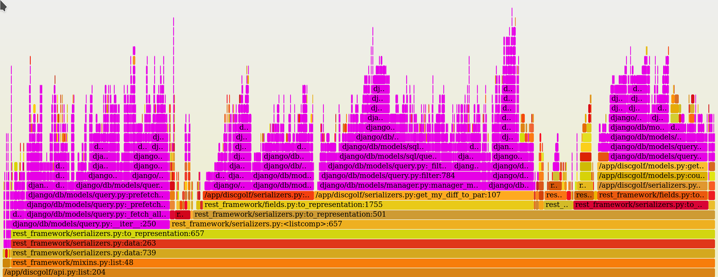
The result is this:

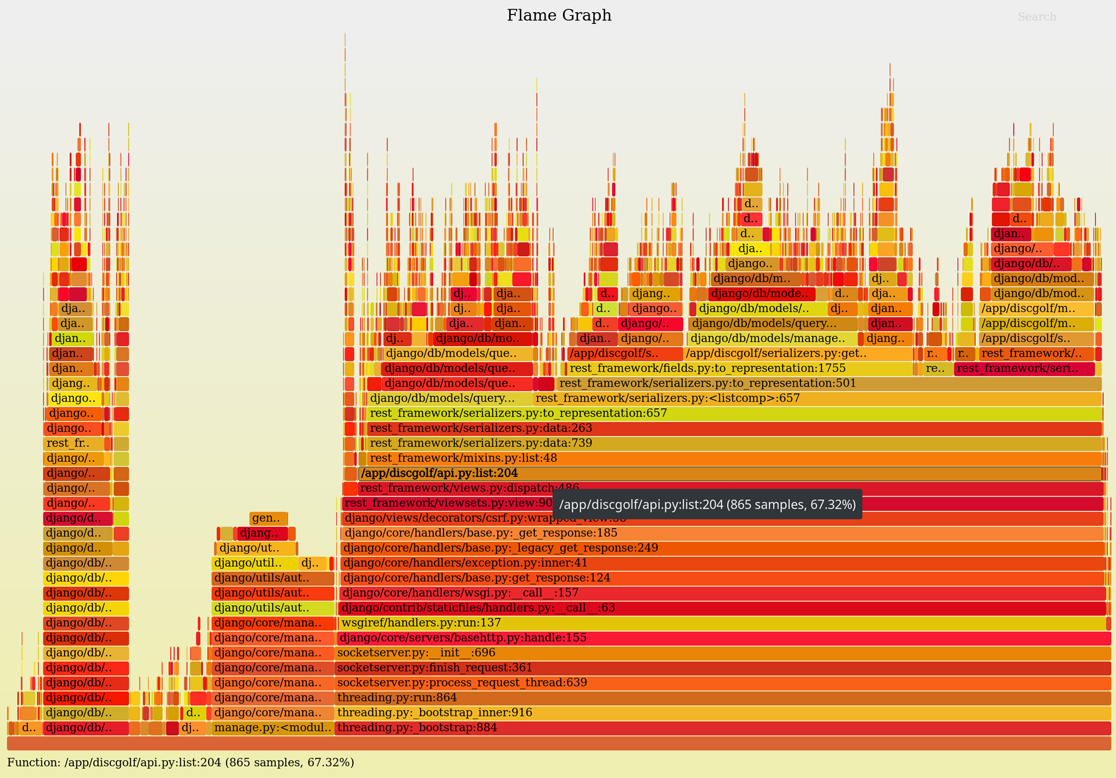
Flamegraphs are pretty intuitive. Starting at the bottom, each ‘layer’ represents a level in the call stack — in other words a child function called by the parent on the level below. The higher the ‘flames’ go, the deeper the call stack was. Width of each box represents the amount of time spent in the corresponding function.

Do note that the X-axis of the graph does not represent time, meaning the graph does not tell you which order the functions were called in.

The wide boxes on top of each other are not very interesting — they represent functions that took long time but only because of something deeper in the call stack, i.e. they didn’t spend that time themselves. The interesting parts are where a single wide box splits into multiple ones, or where a stack of wide boxes suddenly ends, meaning that this function spent a lot of time itself.

Even better, the SVG graphs are interactive — you can hover the boxes to see tooltip with a bit more info, and even click on any box to focus only on it and its descendants. Let’s skip the functions of Django and REST Framework and focus on Discore’s API view itself:

This lets us easily look only at the application code, or only at the module we’re interested in.

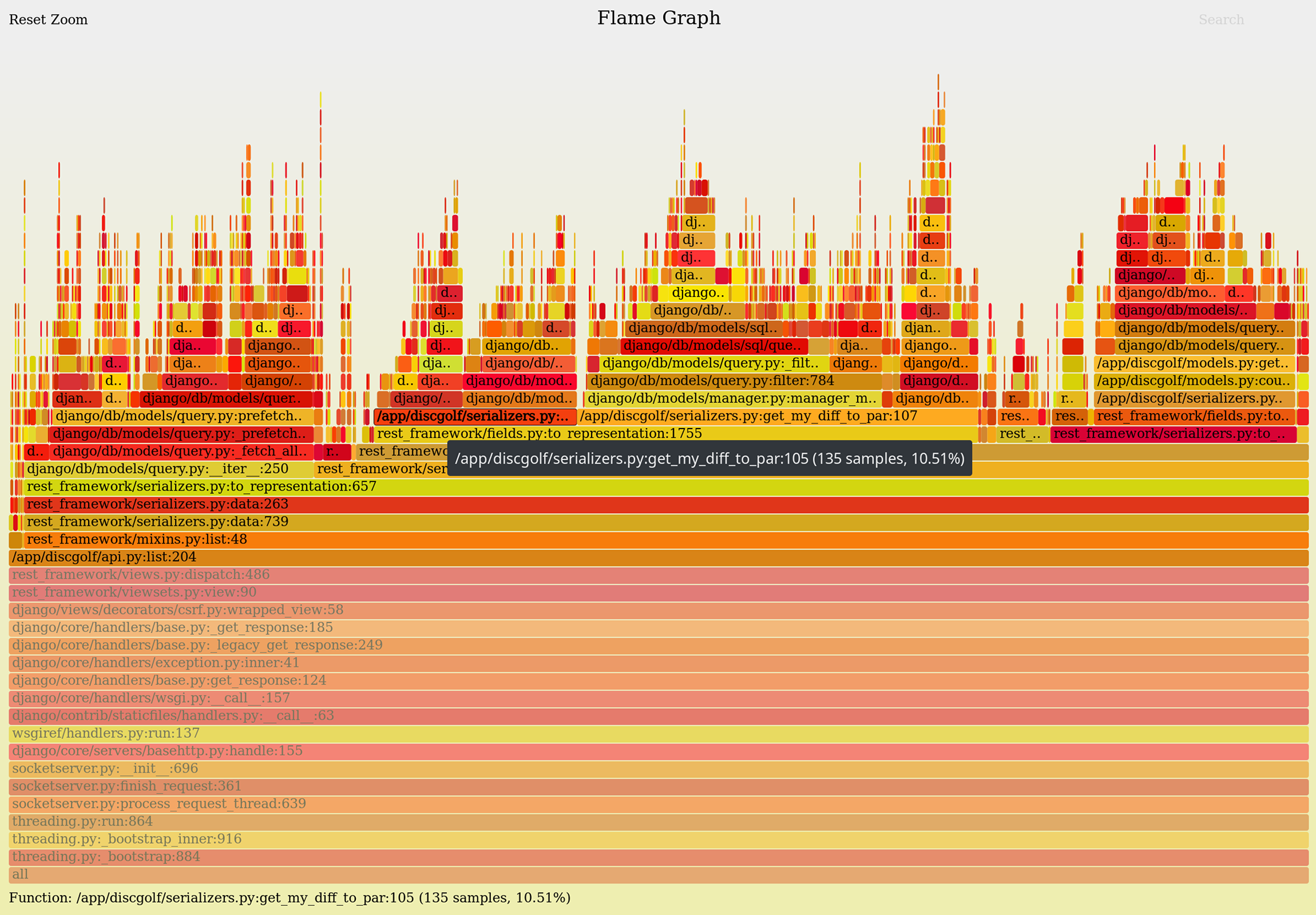
Another nifty trick is search and highlight — again inside the same SVG file. Did you notice the faint “Search” link at the top-right corner? Click it and enter django/db/models/ to highlight Django’s database code. We can see that Discore it spending quite a bit of time dealing with database — looks like a prime spot for optimizations:

Pyflame can also work with code running in Docker containers. You don’t even need to specify any extra flags — just look up your program’s PID (the one in host’s namespace) as usual, and Pyflame handles all the magic. All the above graphs were generated from processes running in Docker.

Conclusions

Hopefully I’ve managed to show a few ways to make finding of performance issues a bit less of a guessing game.

It’s possible to get started by using Python’s built-in capabilities, but I’ve personally found their lack of visualization capabilities to be too limiting. Call graphs make the results much easier to follow, especially when combined with powerful interactive exploring tools such as KCacheGrind.

Statistical profilers such as Pyflame can also be very useful due to their low overhead, making it possible to profile code running in production servers. It also generates interactive flame graphs which once again make it easier to explore where your program’s time is spent.